In this post, I want to share the importance of Fourier series. It has many powerful applications — one of them is that you can draw any shape as a mathematical equation using Fourier series.
To understand the Fourier series better, I used my own picture and recreated it using Fourier series. In this post, I’ll give a basic idea of how to draw an image using Fourier series.
❓What is a Fourier series?
In simple terms, a Fourier series is a sum of sine and cosine waves. The more sine and cosine terms with different frequencies and amplitudes you add to the equation, the more accurately you can draw any complex curve you want.
In mathematical form, we can write it as
$$ f(x) = a_{0} +\sum_{n=1}^\infty a_{n}\cos(nx) +\sum_{n=1}^\infty b_{n}\sin(nx)$$
where,
$a_{0} =\frac{1}{\pi}\int_{-\pi}^{\pi}f(x) \, dx$
$a_{n} =\frac{1}{\pi}\int_{-\pi}^{\pi}f(x)\cos(nx) \, dx$
$b_{n} =\frac{1}{\pi}\int_{-\pi}^{\pi}f(x)\sin(nx) \, dx$
Same equation can written in exponential form as,
$$f(x) = \sum_{n=-\infty}^\infty C_{n}e^{inx}$$
where,
$C_{n}= \frac{1}{2\pi}\int_{-\pi}^{\pi}f(x)e^{(-inx)} \, dx $
In time domain above Fourier equation can be written as
$$f(t) = \sum_{n=-\infty}^\infty C_{n}e^{2\pi i n t}$$
where,
$C_{n}= \int_{0}^{t}f(t)e^{(-2\pi i n t)} \, dt $
Before moving on to image drawing, let’s first understand the steps using a square wave example.
Step 1: Defining the function f(t) of the curve we want to draw using the Fourier series
The square wave can be defined as a function of time, as shown below
$$
f(t) = \begin{cases}
1 & \quad t< 0.5 \\
0 & \quad t= 0.5 \\
-1 & \quad t> 0.5 \\
\end{cases}$$
Step 2: Finding the Fourier coefficients for the function f(t) over the time interval $t \in [0,1]$
Substituting f(t) into the formula for Fourier coefficients:
$$C_{n}= \int_{0}^{0.5}(1)e^{(-2\pi i n t)} \, dt + \int_{0.5}^{1}(-1)e^{(-2\pi i n t)} \, dt $$
Solving this and applying Euler’s identity, we get:
$$
C_{n} = \begin{cases}
0 & \quad if \space n \space even \\
\frac{4}{i 2\pi n} & \quad if \space n \space odd\
\end{cases}$$
Substituting $C_{n}$ into the Fourier series equation and converting the exponential terms into sine and cosine form, the final equation we get:
$$f(t) = \sum_{n=-\infty}^\infty C_{n}e^{2\pi i n t}$$
$$f(t) = \sum_{n=1,3,5..}^\infty \frac{4}{\pi n}\sin{2\pi i n t}$$
By taking enough Fourier coefficients corresponding to different frequencies, we can approximate the square wave. The accuracy of this approximation depends on how many terms (values of n) we include. Below, an example showed how the square wave improves as more Fourier terms(n) are added.
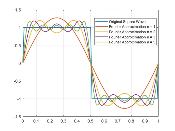
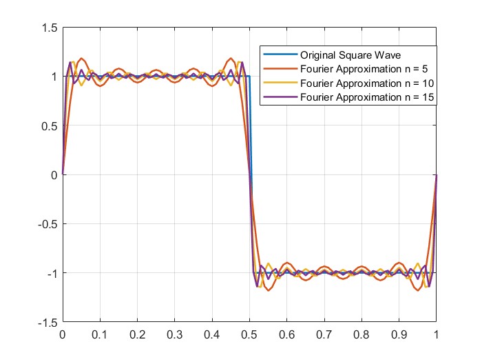
Figure 1: Square wave approximation with Fourier series
Now, Let’s draw the image with the above mentioned steps
In the case of a square wave, we can define f(t) easily. But when it comes to image drawing, it’s not straightforward to define the image as a function of time.
“The image contains many nonlinear curves. Any nonlinear curve behaves like a linear one over a small time interval $(\Delta t)$. Using this simple logic, I discretized the curve into small intervals $(\Delta t)$, which means obtaining the x and y coordinates of the image as discrete points over $\Delta t$ time period. So, within each small interval, I can treat $f(t)$ as a constant.”
So, to discretize the image into x and y coordinates, I used some basic image processing techniques. Below all the steps included from discretization to drawing the image using the Fourier series.
Steps I followed:
Step 1: Extract the discrete points of the image in x and y coordinates. To make the boundary detection easier, I manually drew the boundary in Inkscape and separated it using black and white colors.
Step 2: Interpolated the extracted boundary points at equal intervals $(\Delta t)$ to get a smoother and more accurate representation of the image. Then, I converted the (x, y) coordinates into complex form z=x+iy to calculate the Fourier coefficients easily.
$$f(t) = z|_{t=t+{\Delta t}} = x+iy$$
Here’s the picture for reference.
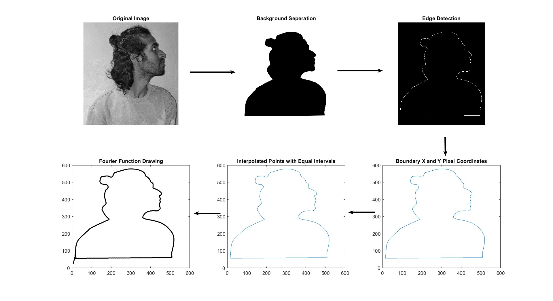
Figure 2: Image Processing Techniques used for Boundary Extraction
Step3: Now I have z(t) as a function of time over small intervals $(\Delta t)$, I used this function as f(t) to calculate the Fourier coefficients for each frequency n. As mentioned in the square wave section, the same equation is used to compute the Fourier coefficients. Which is,
In continuous doman
$$C_{n}= \int_{0}^{t}f(t)e^{(-2\pi i n t)} \, dt $$
In descrete domain
$$C_{n} = \sum_{k=0}^{k=N-1} z(t_{k}) e^{-2\pi i nt_{k}}\Delta t$$
where,
$N = \frac{t}{\Delta t}$
Step 4: Ordering the coefficients from higher to lower for smooth and progressive drawing.
Step 5: Substituting the coefficients into the Fourier series function
$$f(t) = \sum_{n=-\infty}^\infty C_{n}e^{2\pi i n t}$$
I was able to draw my own image, and the result I got is this: