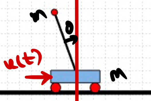
Suppose you are trying to balance a stick on your finger without moving your hand. The stick immediately falls. This happens because the natural tendency of any physical body is to move toward its equilibrium state. Balancing the stick in the upright position is not a stable position.
Figure 1: Inverted pendulum Time Domain Simulation
How do we manage to balance the stick then,
While balancing a stick, we continuously observe its state, and we move our hand accordingly to generate the forces needed to keep it upright.
In this post, we will understand the physics behind balancing a stick and try to balance a simple inverted pendulum using control system basics.
Steps Involved :
- Deriving the dynamics of inverted pendulum model
- Linearizing the dynamics about equilibrium point
- Transfer function modeling
- Finding the appropriate feedback gains for linearize model to balance inverted pendulum model
Dynamics of the Inverted Pendulum Model
Using lagrangian method the the equation of motion of inverted pendulum can be written as,
$$u_{x} = (m+M)\ddot{x} – mL\sin(\theta)(\dot{\theta})^{2} + mL\cos(\theta)\ddot{\theta}$$
$$mL^2\ddot{\theta} – m\ddot{x}L\cos(\theta)-mgL\sin(\theta) = 0$$
The above equation contains nonlinear terms. Any nonlinear system behaves approximately like a linear system over a small operating region. By linearizing the nonlinear system around this region, we can apply linear control methods to easily compute the required feedback gains.
Linearization
To linearize the nonlinear equations, we assume the motion stays close to the upright position. For small angles $\theta$, the following approximations hold:
$$\sin(\theta)≈\theta$$
$$\cos(\theta)≈1$$
assuming $\dot{\theta} ≈ 0$ is near to the equilibrium point
The linearized equations are,
$$u_{x} = (m+M)\ddot{x} + mL\ddot{\theta}$$
$$mL^2\ddot{\theta} – m\ddot{x}L-mgL(\theta) = 0$$
Transfer Function Modeling
By applying the Laplace transform to the above time-domain equations, we convert them into the frequency domain. This gives us the following set of equations:
$$U(S) = (m+M)s^2X(S) + mLs^2\theta(S)$$
$$mL^2s^2\theta(S)-mLs^2X(S)-mgL\theta(S) = 0$$
Combing the above both equations, the final transfer function we get
$$G(S) = \frac{\theta(S)}{U(S)} = \frac{\frac{s^2}{L}}{s^2(1 + \frac{m}{m+M})-\frac{g}{L}}$$
The simple block diagram for this is shown below.
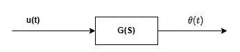
Figure 2: Open Loop Block Diagram
For the above transfer function, if we find the roots of the denominator (known as the poles of the system) and plot them on the complex plane—real axis (x-axis) vs. imaginary axis (y-axis) as shown below, we can see that one pole lies on the right-hand side and the other on the left-hand side of the s-plane.
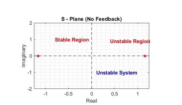
Figure 3: Poles of Inverted Pendulum
According to control system theory, if any pole lies on the right half of the s-plane, the system is unstable.
As mentioned above , we can conclude that holding a stick in the upright position is naturally unstable.
What we can do to make it invert pendulum stable like balancing stick
While balancing a stick, we continuously observe its angle and adjust our hand accordingly. In simple terms, we take feedback of the stick’s angle and modify the input force based on that feedback. Similarly, to balance an inverted pendulum, we can use angle feedback and choose an appropriate gain to balance the pendulum at inverted position.
From a control system perspective, feedback moves system poles from the right half of the s-plane to the left half, which stabilizes the system, since stability requires all poles to lie in the left half-plane.
The block diagram for the system with feedback is
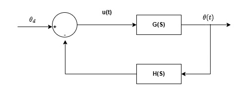
Figure 4: Block Diagram with Feedback
Proportional Feedback
What happens if we take the feedback proportional to the measurement of the angle
$$H(S) = K_{p}$$
$$G(S) = \frac{\frac{s^2}{L}}{s^2(1 + \frac{m}{m+M})-\frac{g}{L}}$$
Figure 5: Root Locus of Simple Inverted Pendulum with proportional Feedback
As we can see from the above animation, as the value of increases from zero, the pole on the right side of the s-plane moves toward the left but settles on the imaginary axis of the s-plane. As a result, the system becomes marginally stable and oscillates about the desired angle(shown in fiugre-1).
Using only proportional feedback we were unable to stabilize the inverted pendulum.
Proportional and Derivative Feedback
What if we also take the rate of change of the angle as feedback? Since the angular rate determines how the angle will evolve next, controlling it gives us better control over the system’s angle.
$$G(S) = \frac{\frac{s^2}{L}}{s^2(1 + \frac{m}{m+M})-\frac{g}{L}}$$
$$H(S) = K_{p} + K_{d}s $$
Figure 5: Root Locus of Simple Inverted Pendulum with Proportional and Derivative Feedback
As seen in the above animation, after introducing proportional–derivative (PD) feedback, increasing and moves all system poles completely into the left half of the s-plane. As a result in the Figure 1 animation, we can see that the pendulum is fully stabilized at the inverted position, as desired.