In this project, I am showing how to write the name “Robo” using 2R manipulator in Matlab. A 2R manipulator is a two degree of freedom robotic manipulator with revolute joints. The reason for choosing the 2R manipulator is that it is easy to understand and implement.
To write the name “Robo,” first we need to define the waypoints in the shape of the letters ‘R’, ‘o’, ‘b’, and ‘o’, as shown in the figure above. After defining the waypoints, the next step is to determine the trajectory that the manipulator must follow between two waypoints.
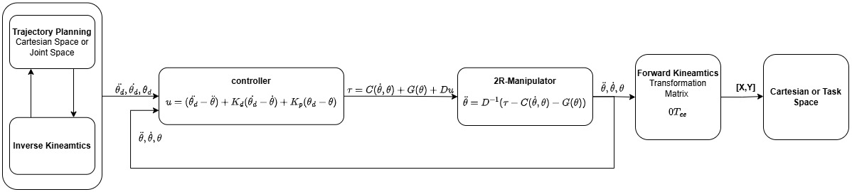
Steps involved to move the 2R-Manipulator from one waypoint to another way point.
- Trajectory planning between two waypoints in cartesian space or joint space, referred to as the start and goal position.
Inverse kinematics converts Cartesian space coordinates in [x, y] to joint space coordinates [θ1, θ2].
- Controller to track the desired joint space trajectories, which are obtained from inverse kinematics.
- Forward Kinematics converts joint space coordinates [θ1, θ2] into Cartesian space coordinates [x, y].
The following block diagram provides an overview of the steps involved in moving the manipulator from the start position to the goal position.
Trajectory Planning
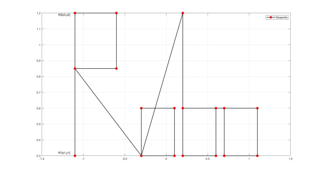
For example, to write the letter “R,” the initial movement must be from R1 [x1,y1] to R2 [x2,y2] in a vertical direction. A path must be established between R1 and R2 to move the end effector from R1 to R2, which can be called as trajectory planning.
For trajectory planning, there are two options.
- One method involves designing trajectory between R1[x1,y1] and R2[x2,y2] in cartesian space and the inverse kinematics $[\theta_{1}, \theta_{2}]$ is calculated at each discrete point. This approach is known as task space trajectory planning.
- Another method involves designing trajectory in joint space$[\theta_{1}, \theta_{2}]$. Computing $[\theta_{1}, \theta_{2}]$ using inverse kinematics at R1[x1,y1] and R2[x2,y2] and then interpolating those values using a polynomial equation. This approach is referred to as joint space trajectory planning.
In this simulation joint space trajectory planning was used. Joint space coordinates $[\theta_{1},\theta_{2}]$ were calculated using the inverse kinematics at R1 and R2 waypoints and interpolated using following polynomial equation
$$\theta(t) = a_{0} + a_{1}t + a_{2}t^{2} + a_{3}t^{3}$$
where the boundary conditions were,
$\theta(t_{0}) = \theta_{0}$, $\theta(t_{f}) = \theta_{f}$
$\dot{\theta}(t_{0}) = \dot{\theta}_{0}$, $\dot{\theta}(t_{f}) = \dot{\theta}_{f}$
Inverse Kinematics
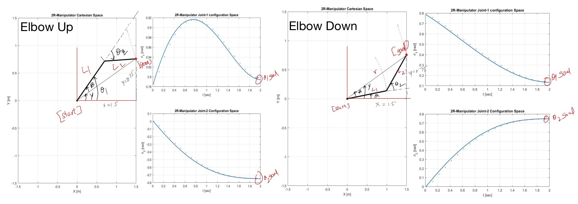
Inverse kinematics can be calculated using analytical and graphical methods, or you can use the Jacobian approach. Here, graphical method was used, because it is easy to implement and involves no complexity.
Using the graphical method, there are two possible solutions to reach the goal position: elbow-up and elbow-down. The only difference between these positions is the change in sign.
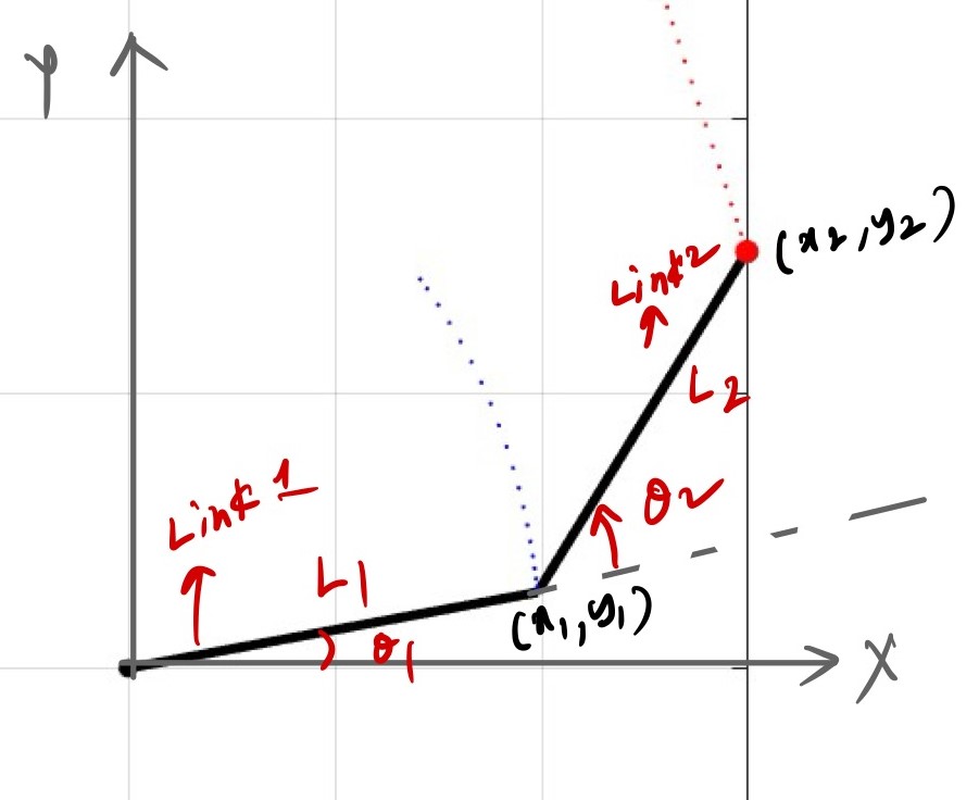
In the graphical method, $\theta_{1}$ and $\theta_{2}$ are expressed as
$$ \theta_{2} = \pm \cos^{-1}(\frac{(x^2 + y^2)-(L_{1}^2 + L_{2}^{2})}{2L_{1}L_{2}}) $$
$$ \beta = \tan^{-1}(\frac{L_{2}\sin\theta_{2}}{L_{1} + L_{2}\cos{\theta}_{2}})$$
$$\gamma = \tan^{-1}(\frac{y}{x}) $$
$$ \theta_{1} = \gamma \pm \beta $$
Manipulator Dynamics
The equation of motion for a manipulator can be derived using the Lagrangian method. The Euler-Lagrange equation is given by
$$\frac{d}{dt}(\frac{\partial L}{\partial \dot{\theta_{i}}}) – \frac{\partial L}{\partial \theta_{i}} = \tau_{i} $$
where $L = K-P$
K is the kinetic energy of the system
P is the potential energy system
$\theta_{i}$ is the generalized coordinate
$\tau_{i}$ is the generalized force or torque.
The position of link1 and link2 w.r.t global reference frame is
$$ x_{1} = L_{1}\cos(\theta_{1}) $$
$$ y_{1} = L_{1}\sin(\theta_{1}) $$
$$ x_{2} = L_{1}\cos(\theta_{1}) + L_{2}\cos(\theta_{1}+\theta_{2}) $$
$$ y_{2} = L_{1}\sin(\theta_{1}) + L_{2}\sin(\theta_{1}+\theta_{2}) $$
The velocity w.r.t global reference frame is
$$ \dot{x_{1}} = L_{1}\cos(\theta_{1})\dot{\theta_{1}} $$
$$\dot{y_{1}} = L_{1}\sin(\theta_{1})\dot{\theta_{1}} $$
$$ \dot{x_{2}} = L_{1}\cos(\theta_{1})\dot{\theta_{1}} + L_{2}\cos(\theta_{1}+\theta_{2}) (\dot{\theta_{1}} + \dot{\theta_{2}}) $$
$$ \dot{y_{2}} = L_{1}\sin(\theta_{1})\dot{\theta_{1}} + L_{2}\sin(\theta_{1}+\theta_{2}) (\dot{\theta_{1}} + \dot{\theta_{2}}) $$
The Kinetic energy of the mass m1 and m2 are
$$ K = K_{1} + K_{2}$$
$$ K = \frac{1}{2}m_{1}(\dot{x_{1}}^2 + \dot{y_{1}}^2 ) + \frac{1}{2}m_{2}(\dot{x_{2}}^2 + \dot{y_{2}}^2 )$$
The potential energy of mass m1 and m2 are
$$ P = P_{1} + P_{2}$$
$$ P = m_{1}gy_{1} + m_{2}gy_{2}$$
By substituting the K and P variables into L and applying the Euler-Lagrange equation, the equations of motion for Link 1 and Link 2 are:
$$ \tau_{1} = (m_{1} + m_{2})l_{1}^2 \ddot{\theta_{1}} + I_{1}\ddot{{\theta_{1}}} + m_{2}l_{2}^2(\ddot{{\theta_{1}}} + \ddot{{\theta_{2}}}) + m_{2}l_{1}l_{2}(2\ddot{{\theta_{1}}}+\ddot{{\theta_{2}}})\cos(\theta_{2})-m_{2}l_{1}l_{2}\dot{\theta_{2}}(2\dot{\theta_{1}}+\dot{\theta_{2}})\sin(\theta_{2}) + m_{1}gl_{1}\cos\theta_{1} + m_{2}g(l_{1}\cos\theta_{1} + l_{2}\cos(\theta_{1} + \theta_{2}))$$
$$ \tau_{2} = m_{2}l_{2}^2(\ddot{\theta_{1}} + \ddot{\theta_{2}}) + m_{2}l_{1}l_{2} \ddot{\theta_{1}}\cos\theta_{2} – m_{2}l_{1}l_{2}\dot{\theta_{1}}\dot{\theta_{2}}\sin{\theta_{2}} + m_{2}l_{1}l_{2}\dot{\theta_{1}}(\dot{\theta_{1}} + \dot{\theta_{2}})\sin{\theta_{2}} + m_{2}gl_{2}\cos(\theta_{1} + \theta_{2}) + I_{2}(\ddot{\theta_{1}} + \ddot{\theta_{2}})$$
Here,
$m_{1}$,$m_{2}$ are the mass of the link1 and link2
$I_{1}$,$I_{2}$ are the moment of inertia of the link1 and link2
$l_{1}$,$l_{2}$ are the length of the link1 and link2
Writing the above equations in matrix form
$$D(\ddot{\theta}) + C(\dot{\theta},\theta) +G(\theta) = \tau$$
Where,
D is nxn matrix, n is degrees of freedom of manipulator
C nx1 Coriolis and centrifugal component matrix
G nx1 gravitational component matrix
$\tau = [\tau_{1}\space\tau_{2}]^{T}$
In the case of a 2R manipulator with n = 2, the terms $D(\ddot{\theta})$, $C(\dot{\theta}, \theta)$, and $G(\theta)$ can be expressed as:
$$ D(\ddot{\theta}) = \begin{bmatrix}
I_{1} + (m_{1}+m_{2})l_{1}^{2}+m_{2}l_{2}^{2}+2m_{2}l_{1}l_{2}\cos(\theta_{2}) & m_{2}l_{2}^2+m_{2}l_{1}l_{2}\cos(\theta_{2}) \\
I_{2}+m_{2}l_{2}^2 + m_{2}l_{1}l_{2}\cos(\theta_{2}) &I_2+m_{2}l_{2}^2
\end{bmatrix}
$$
$$ C(\dot{\theta},\theta) = \begin{bmatrix}
-m_{2}l_{1}l_{2}{\dot{\theta_{2}}(2\dot{\theta_{1}}+\dot{\theta_{2}})}\sin(\theta_{2}) \\
-m_{2}l_{1}l_{2}\dot{\theta_{1}}\dot{\theta_{2}}\sin(\theta_{2})+m_{2}l_{1}l_{2}\dot{\theta_{1}}(\dot{\theta_{1}}+\dot{\theta_{2}})\sin(\theta_{2})
\end{bmatrix}
$$
$$ G(\theta) = \begin{bmatrix}
(m_{1}+m_{2})gl_{1}\cos(\theta_{1})+m_{2}gl_{2}\cos(\theta_{1}+\theta_{2})) \\
m_{2}gl_{2}\cos(\theta_{1}+\theta2)
\end{bmatrix}
$$
Controller
$$u = (\ddot{\theta_{d}}-\ddot{\theta}) + K_{d}(\dot{\theta_{d}}-\dot{\theta}) + K_{p}({\theta_{d}}-{\theta})$$
$K_{p}$ is the proportional gain
$K_{r}$ is the rate gain
$\ddot{\theta_{d}}$,$\dot{\theta_{d}}$,$\theta_{d}$ are the desired the angular acceleration, angular velocity and angle calculated using inverse kinematics
$\ddot{\theta}$,$\dot{\theta}$,$\theta$ are the actual angular acceleration, angular velocity and angle
To linearize the system the input torque $\tau$ can be written as
$$\tau = C(\dot{\theta},\theta) +G(\theta) + D(\ddot{\theta})u$$
The reason behind linearizing a nonlinear system is to use linear system controller methods to calculate the $K_{p}$ and $K_{d}$ gains.
Forward Kinematics
The forward kinematics is formulated using Denavit–Hartenberg (D-H) parameters. According to the D-H convention, the position and orientation of any robot in space can be defined using four parameters, which are
$\theta_{i}$ – angle between $x_{i-1}$ and $x_{i}$ about $z_{i-1}$ .
$d_{i}$ – distance along $z_{i-1}$ from $i-1$ axes to the intersection of $x_{i}$ and $z_{i-1}$ axes
$a_{i}$ – distance along $x_{i}$ from $i$ axes to the intersection of $x_{i}$ and $z_{i-1}$ axes
$\alpha_{i}$ – angle between $z_{i-1}$ and $z_{i}$ about $x_{i}$.
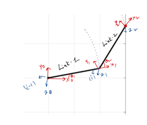
D-H Parameters
| Link(i) | $\theta_{i}$ | $d_{i}$ | $a_{i}$ | $\alpha_{i}$ |
| 1 | $\theta_{1}$ | $0$ | $L_{1}$ | $0$ |
| 2 | $\theta_{2}$ | $0$ | $L_{2}$ | $0$ |
Transformation matrix from base link to end effector
$0T_{ee}=$
$$\begin{bmatrix}
\cos(\theta_{1}) & -\sin(\theta_{1}) & L_{1}\cos(\theta_{1}) \\
-\sin(\theta_{1}) & \cos(\theta_{1}) & L_{1}\sin(\theta_{1}) \\
0 & 0 & 1
\end{bmatrix}
\begin{bmatrix}
\cos(\theta_{2}) & -\sin(\theta_{2}) & L_{2}\cos(\theta_{2}) \\
-\sin(\theta_{2}) & \cos(\theta_{2}) & L_{2}\sin(\theta_{2}) \\
0 & 0 & 1
\end{bmatrix}$$
$$x_{2} = 0T_{ee(3,1)}$$
$$y_{2} = 0T_{ee(3,2)}$$